Project Overview
Rectifying some crooked paintings, and stitching together a keyboard.
Computing Homography Matrix
The goal is to find a homography matrix that transforms points from one image to another. The relationship between points can be expressed in homogeneous coordinates as:
This implies that \( w = g \cdot p_1 + h \cdot p_2 + 1 \). We can substitute this into the relations:
These equations are not linear in \(p_1\) and \(p_2\), but they are linear in \(a, b, c, d, e, f, g, h\). By stacking this into matrix form, we obtain:
The left data matrix and right data vector are extended by 2 rows for each additional correspondence. We require at least 4 correspondences between the two images for the system to not be underdetermined.
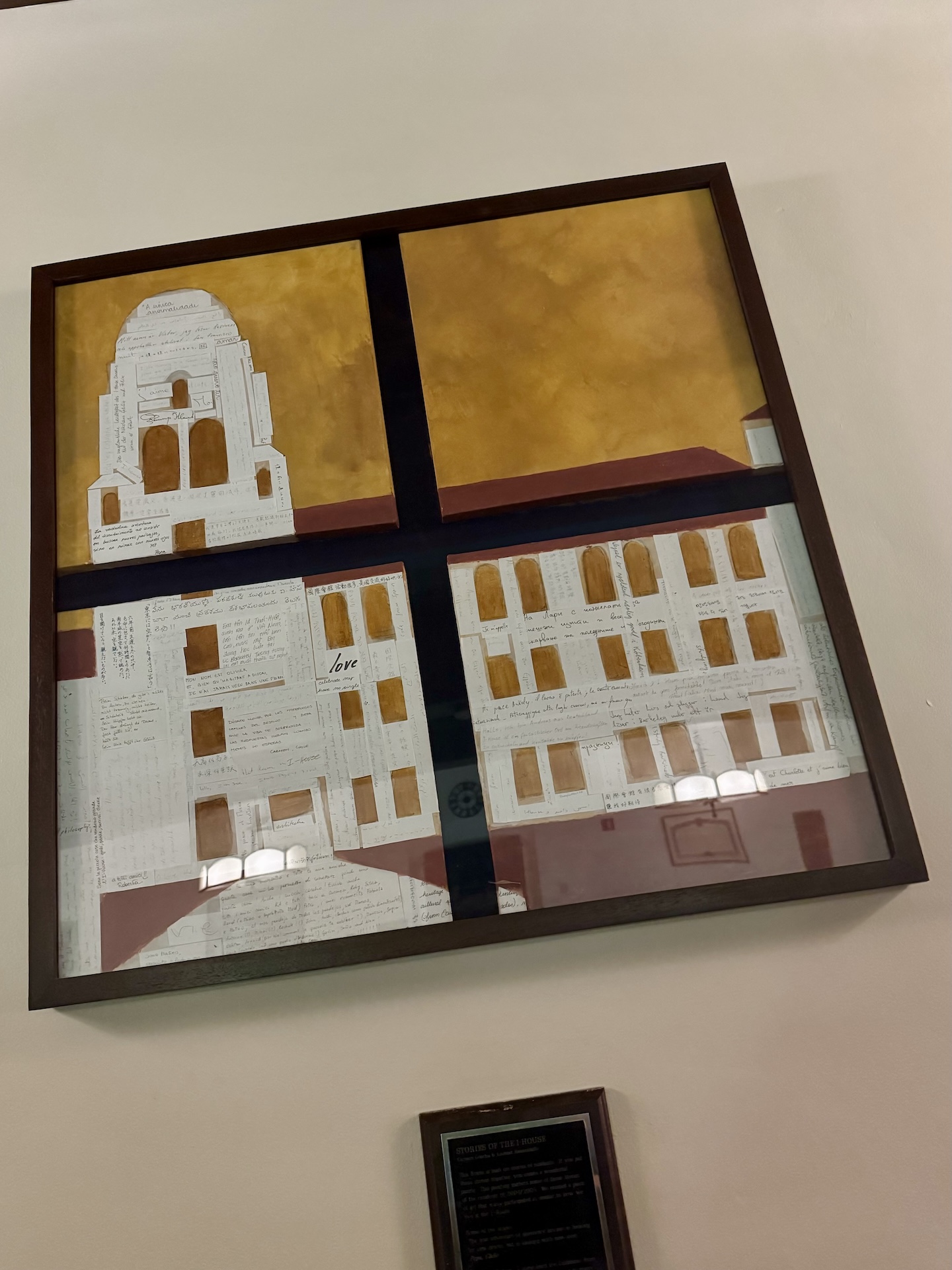
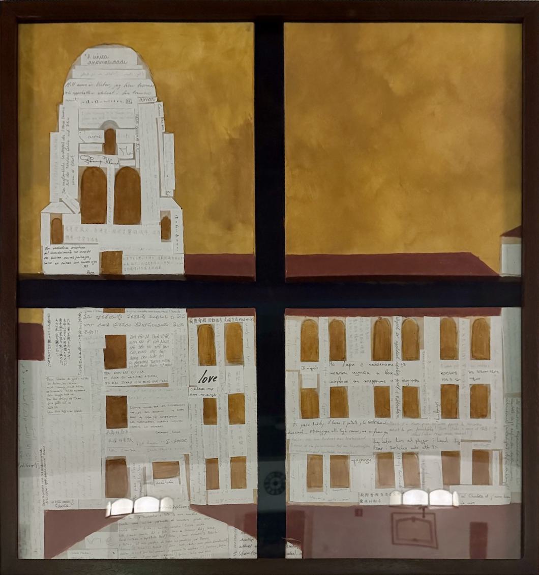
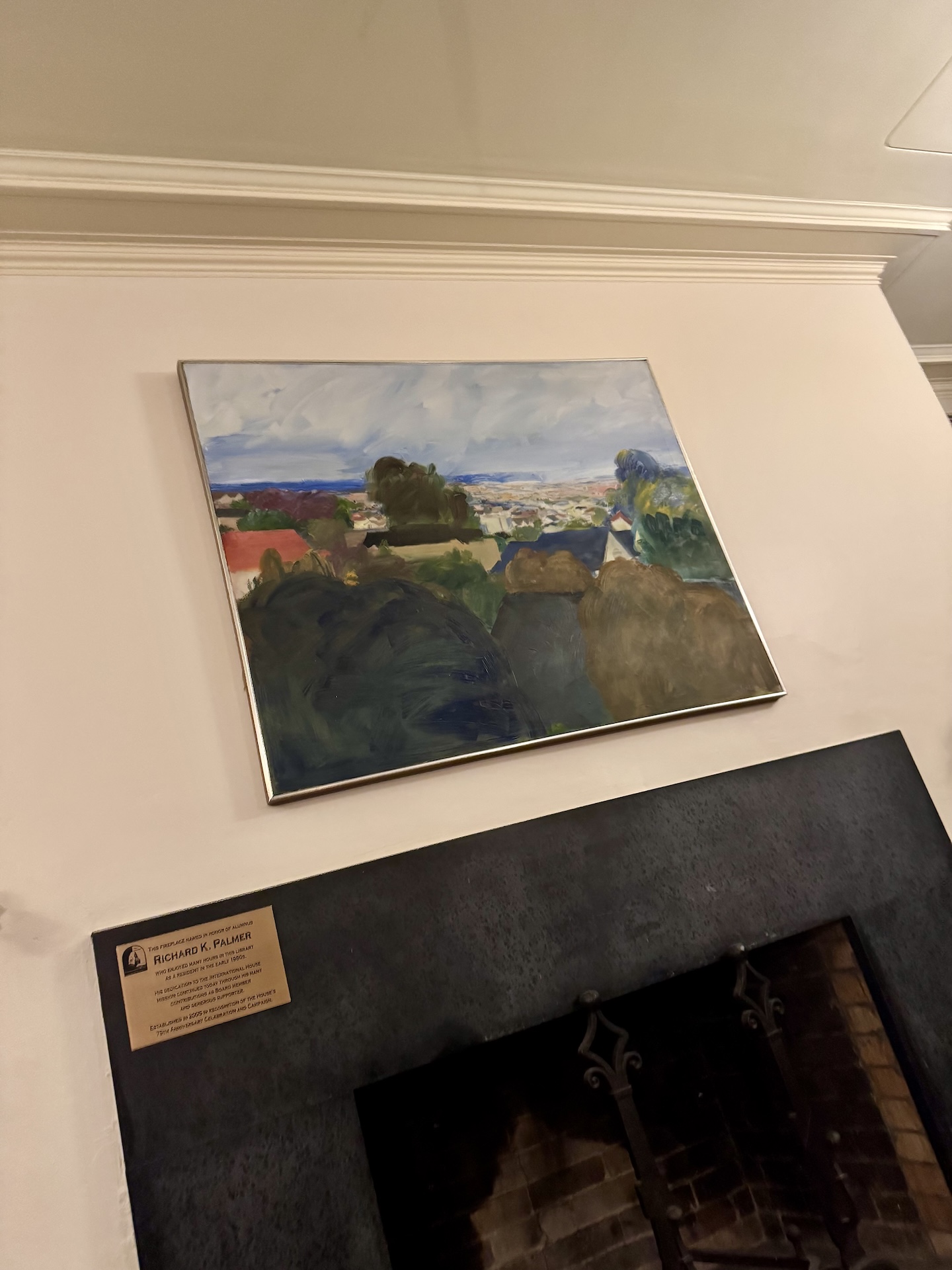
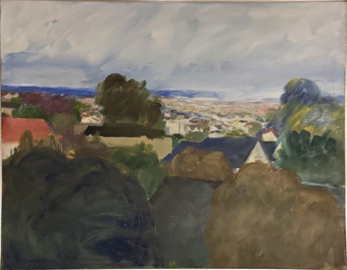
Rectifying Images
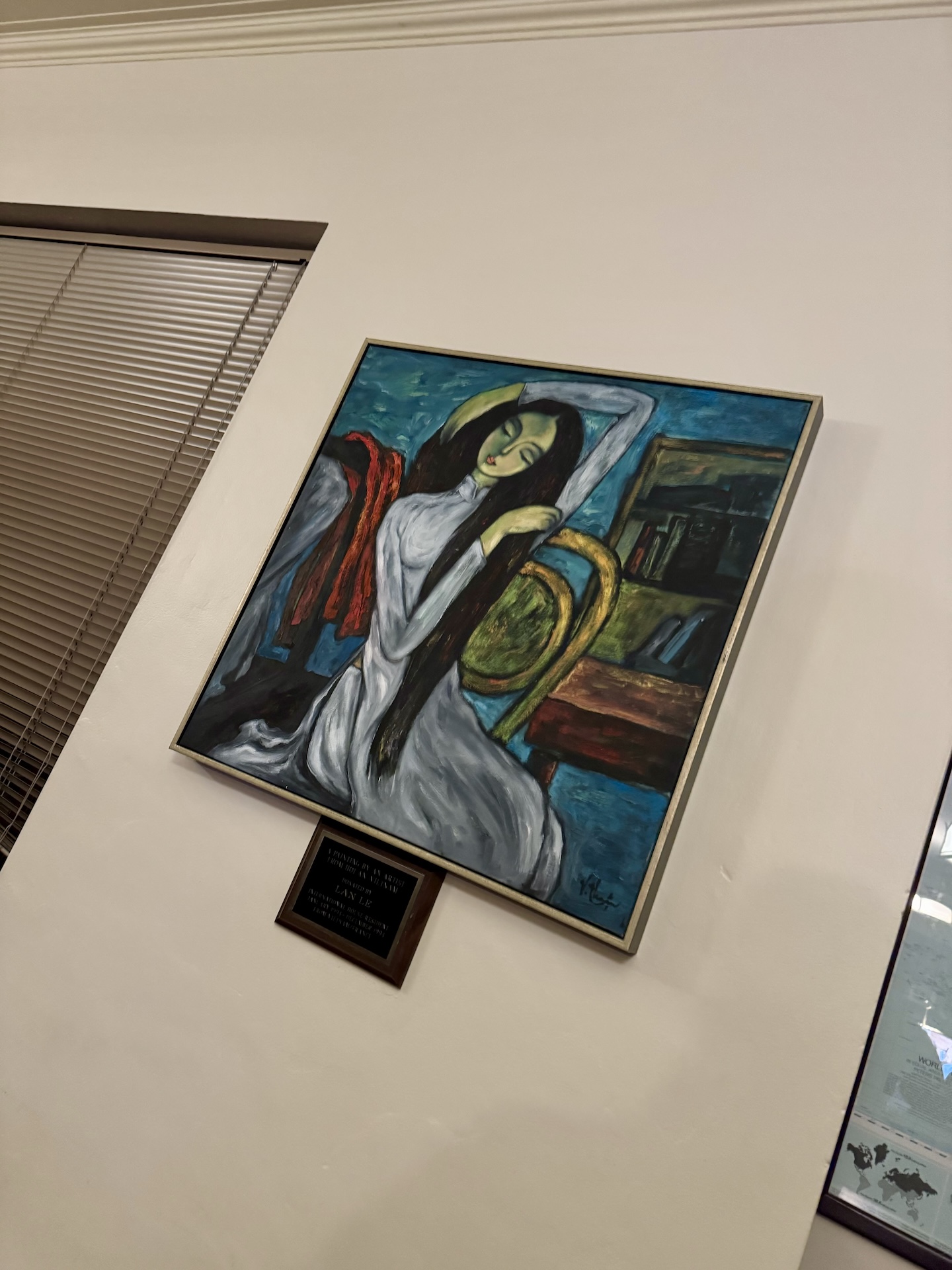
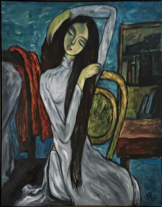
Creating the Mosaic Manually
While the results aren't quite what one would expect, for this section of the project, I took 3 images of my keyboard while pivoting my phone on the axis of the camera hub. I then warped the left and right images and stitched them to the middle image and blended.
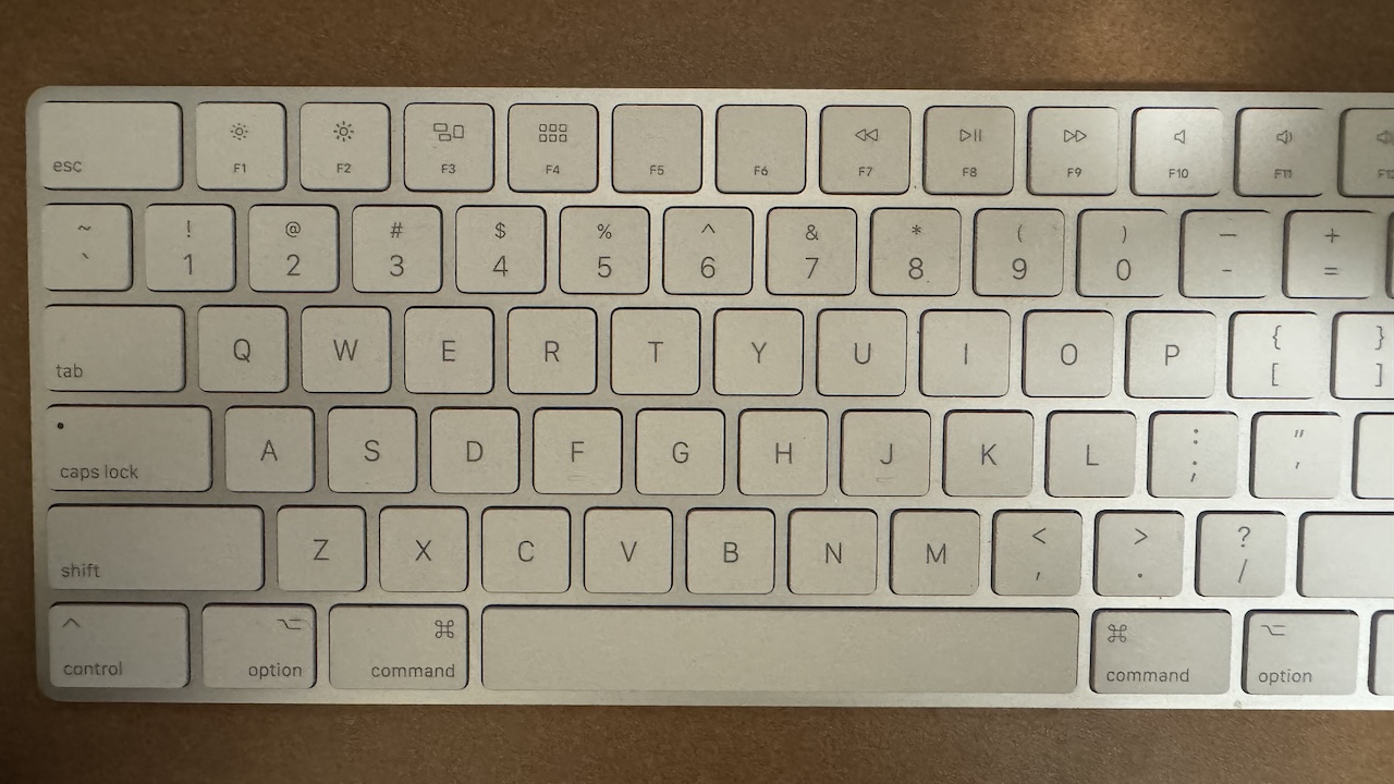
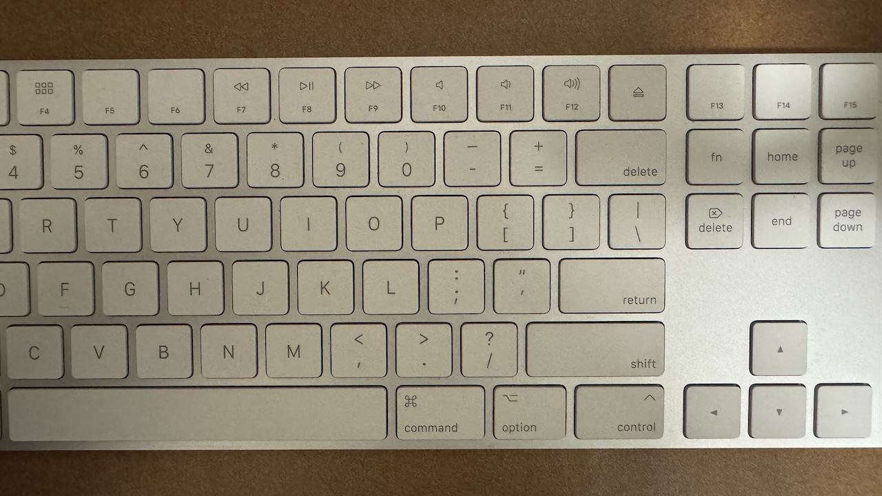
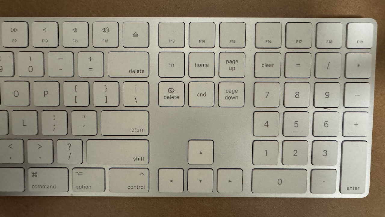
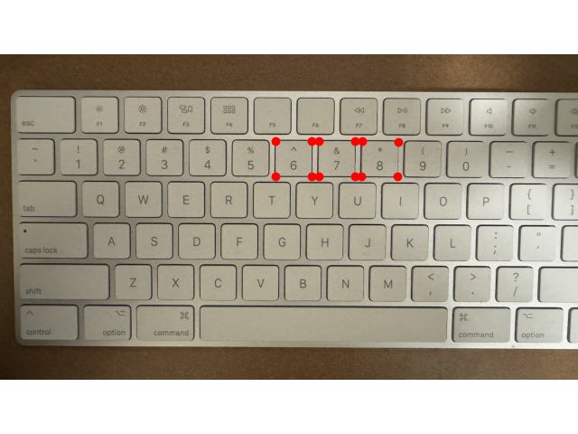
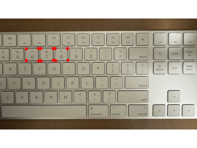
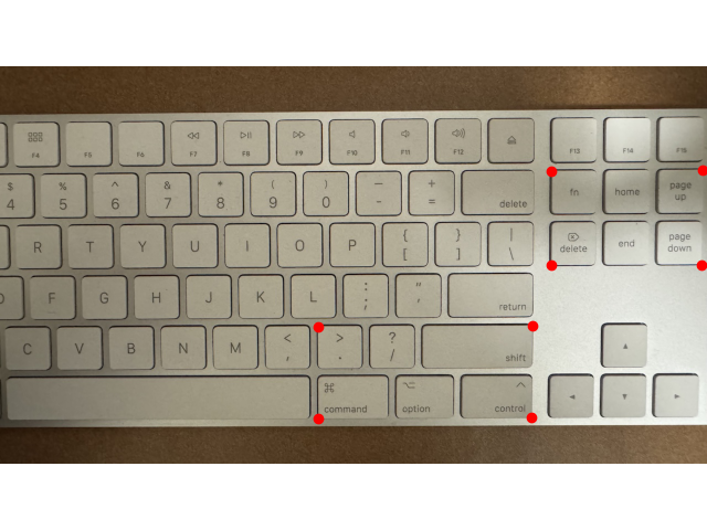
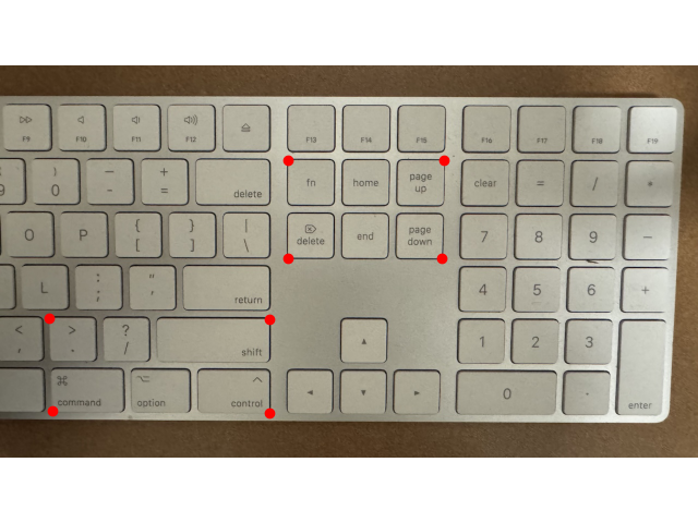
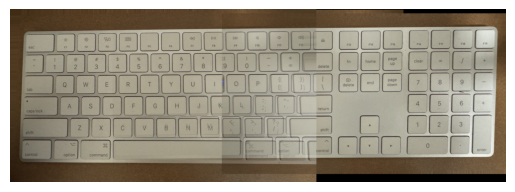
Due to some lighting imbalance, the end result of my mosaic is not quite as clean as I would like While the alignment and image rectification is decent for the left and right images, I believe that an accident change in lighting caused an issue with the alignment of the middle image component.
Harris Corner Detection
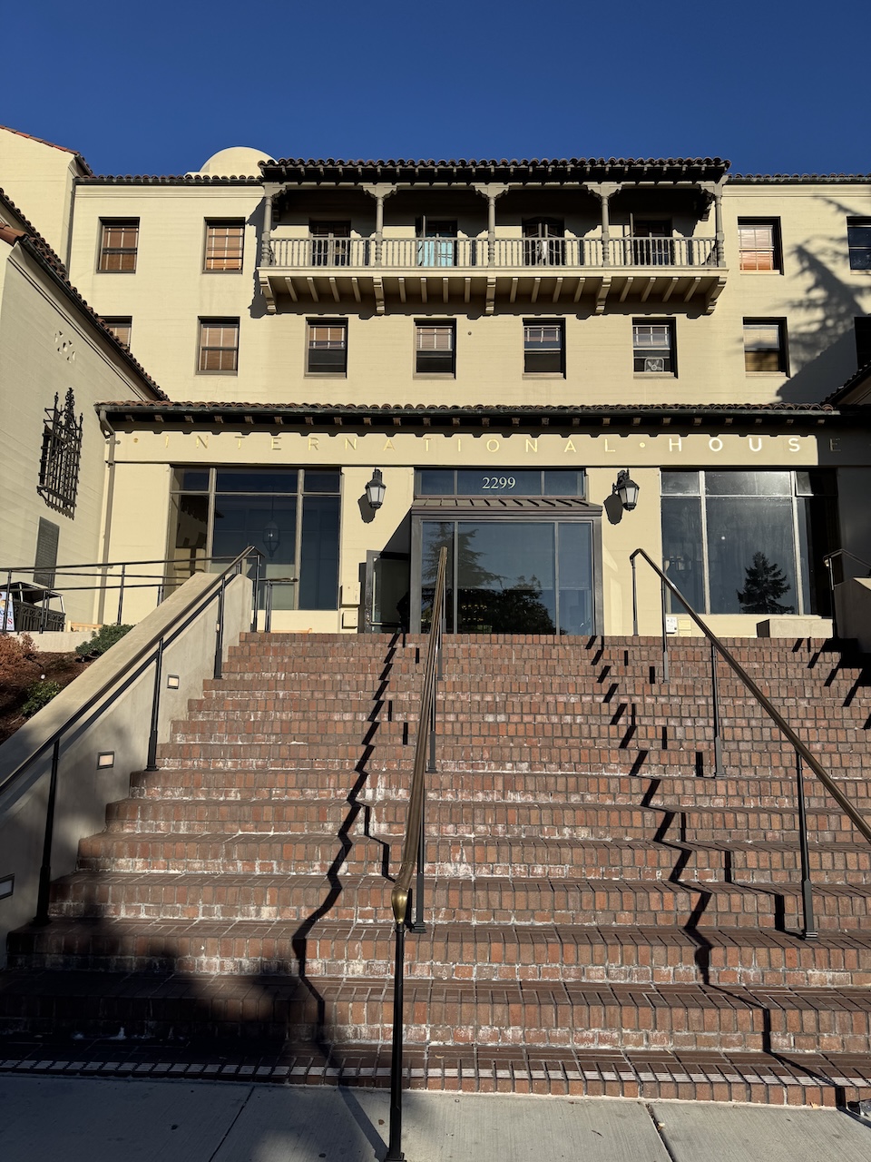
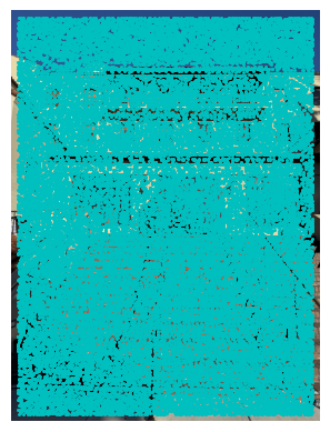
Utilizing the provided code for Harris corner detection, I ran that code and plotted these images, which list all possible corner coordinates. This yields far too many corners for it to be of any use. Thus, in the next section, ANMS is used to reduce the number of potential keypoints to the ones that represent the strongest, or best-fit, corners. These corners are identitified throughout the image
Adaptive Non-Maximal Suppression
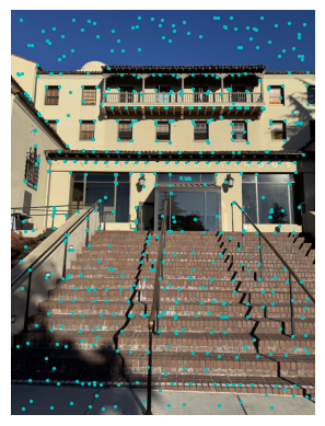
Identifying all the Harris interest points typically results in a dense set of points. To reduce this set to a more useful number, I utilized the Adaptive Non-Maximal Suppression (ANMS) algorithm as per the geuidelines. The goal was to select interest points that were both well-distributed and had a strong corner response.
The algorithm operates by first sorting the detected Harris points based on their response strength. For each point \( x_i \), I identified all other points \( x_j \) with a greater response strength and multiplied each response by a factor of \( c_{\text{robust}} \) (which was set to 0.9). I then computed the distance \( r_i \) between each point \( x_i \) and its closest stronger point. This distance calculation can be expressed by the following equation:
\( r_i = \min_j \| x_i - x_j \|, \quad \text{subject to} \quad f(x_i) < c_{\text{robust}} \cdot f(x_j), \quad x_j \in \mathcal{I} \)
where \( f(x) \) denotes the corner response strength of point \( x \), and \( \mathcal{I} \) is the set of all detected points.
After calculating this list of distances, I sorted the points and selected the strongest ones that were furthest from their neighbors. In this case, I chose to keep 500 points as described in the paper, ensuring a balance between point density and distribution.
Feature Extraction
According to the paper, subsampling a larger patch around an interest point to create feature descriptors enhances their overall effectiveness. However, to prevent aliasing, it is essential to appropriately blur the image before this step, ensuring that frequencies beyond the Nyquist limit are removed prior to subsampling. For this simplified implementation, an axis-aligned patch is used, and the feature detection occurs only at a single level of the Gaussian pyramid.
Feature Matching
After extracting these basic features, the pairwise distances between features in one image and those in another are calculated. The ratio of the error between the closest and second-closest neighbors (commonly referred to as Lowe's ratio) is then computed and used as a threshold. This approach provides better discrimination than relying solely on the distance to the nearest neighbor.
RANSAC (RAndom SAmple Consensus)
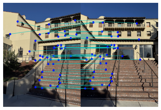
Getting matches between paired images isn't enough since not all matches are accurate. Thus, the RANSAC algorithm was used to identify inliers within the set of matches and ensure only spatially accurate matches are kept. Essentially, RANSAC gets rid of false positives.
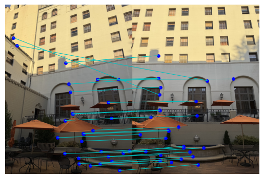
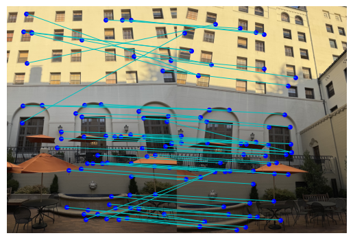
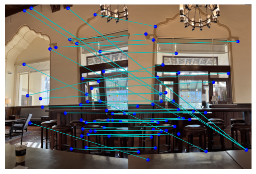
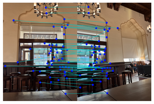
Below is the visualization of the matches after feature extraction, matching, and RANSAC-ing.
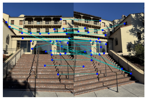
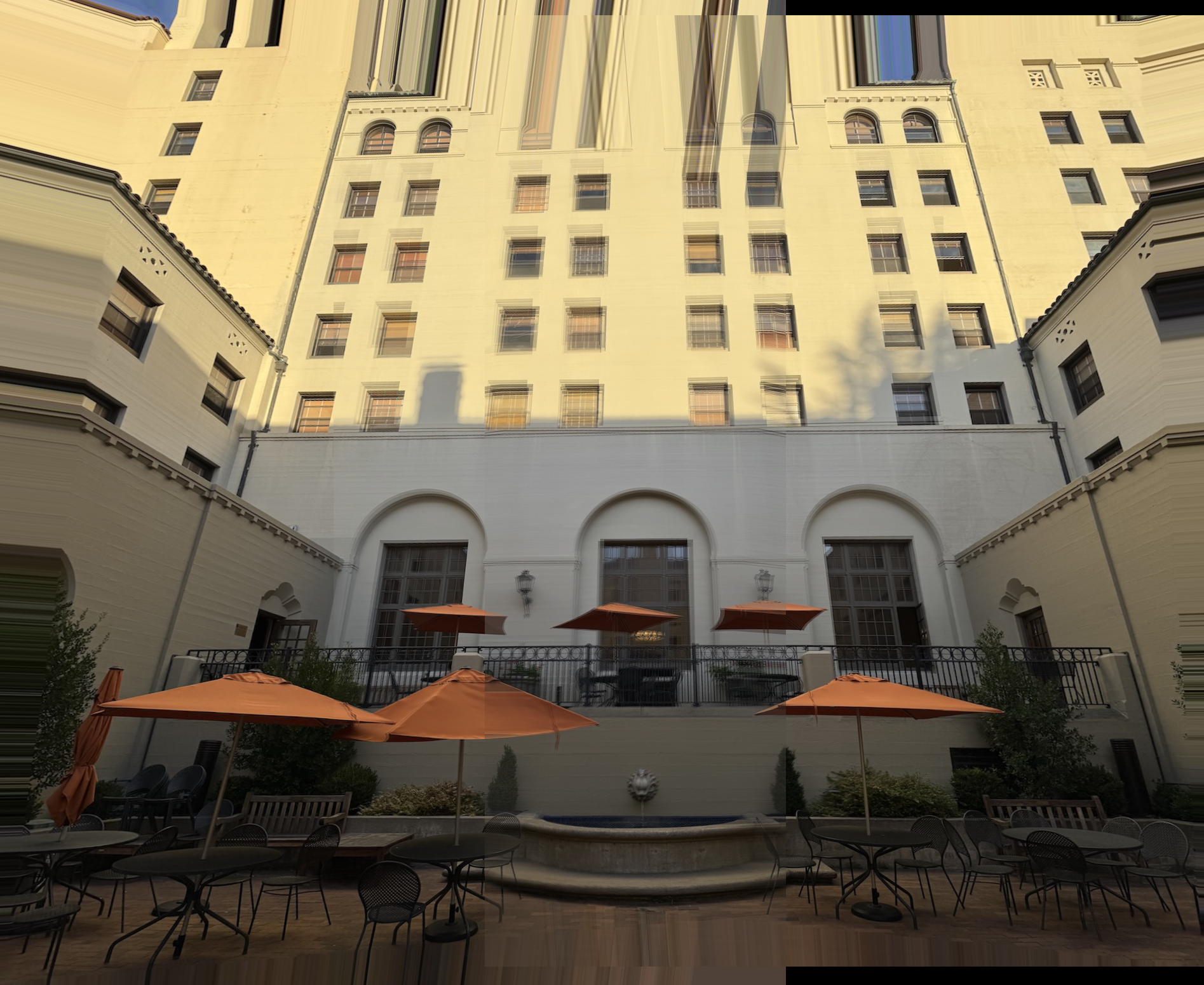
This process results in the following panorama for ihouse.
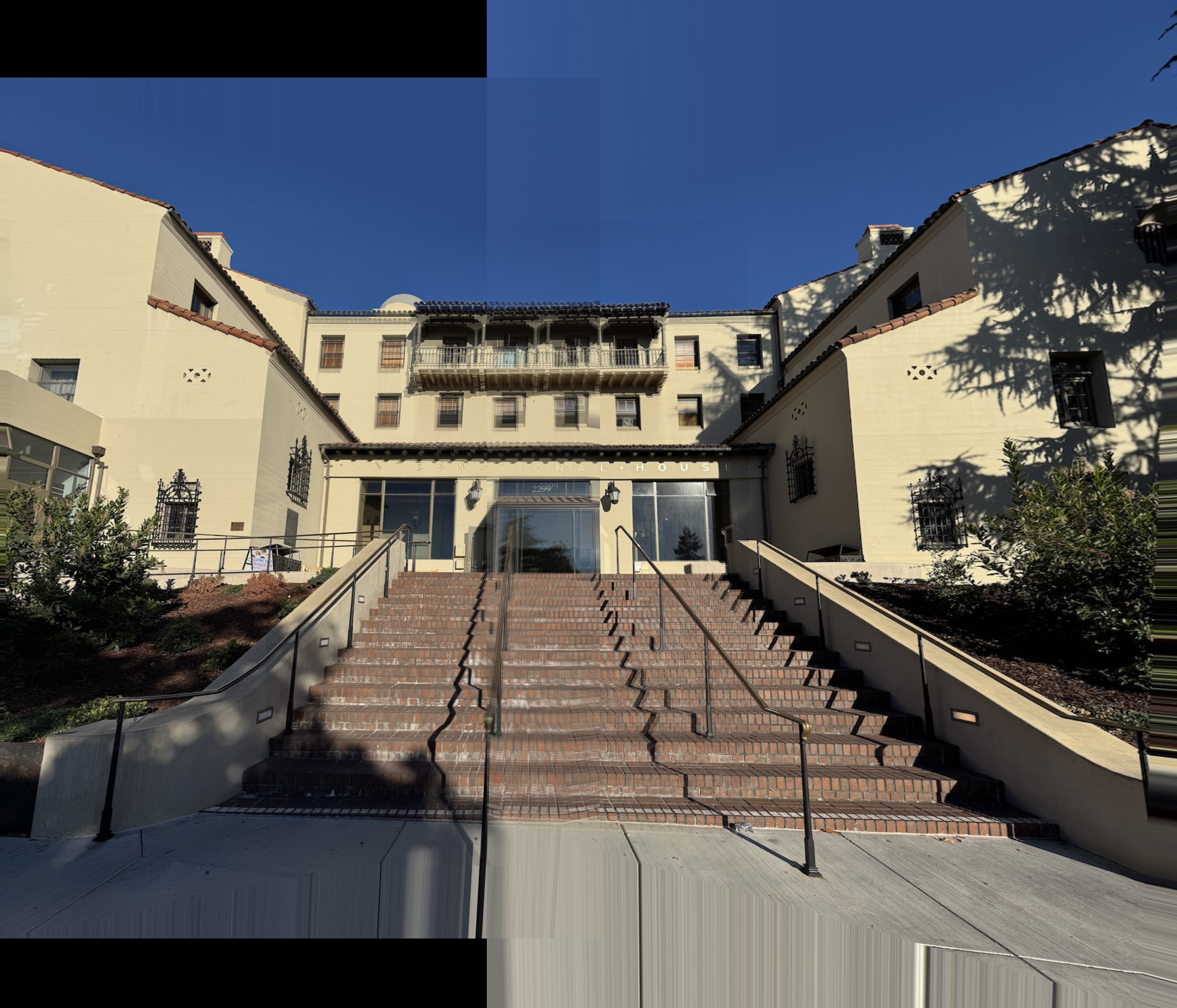
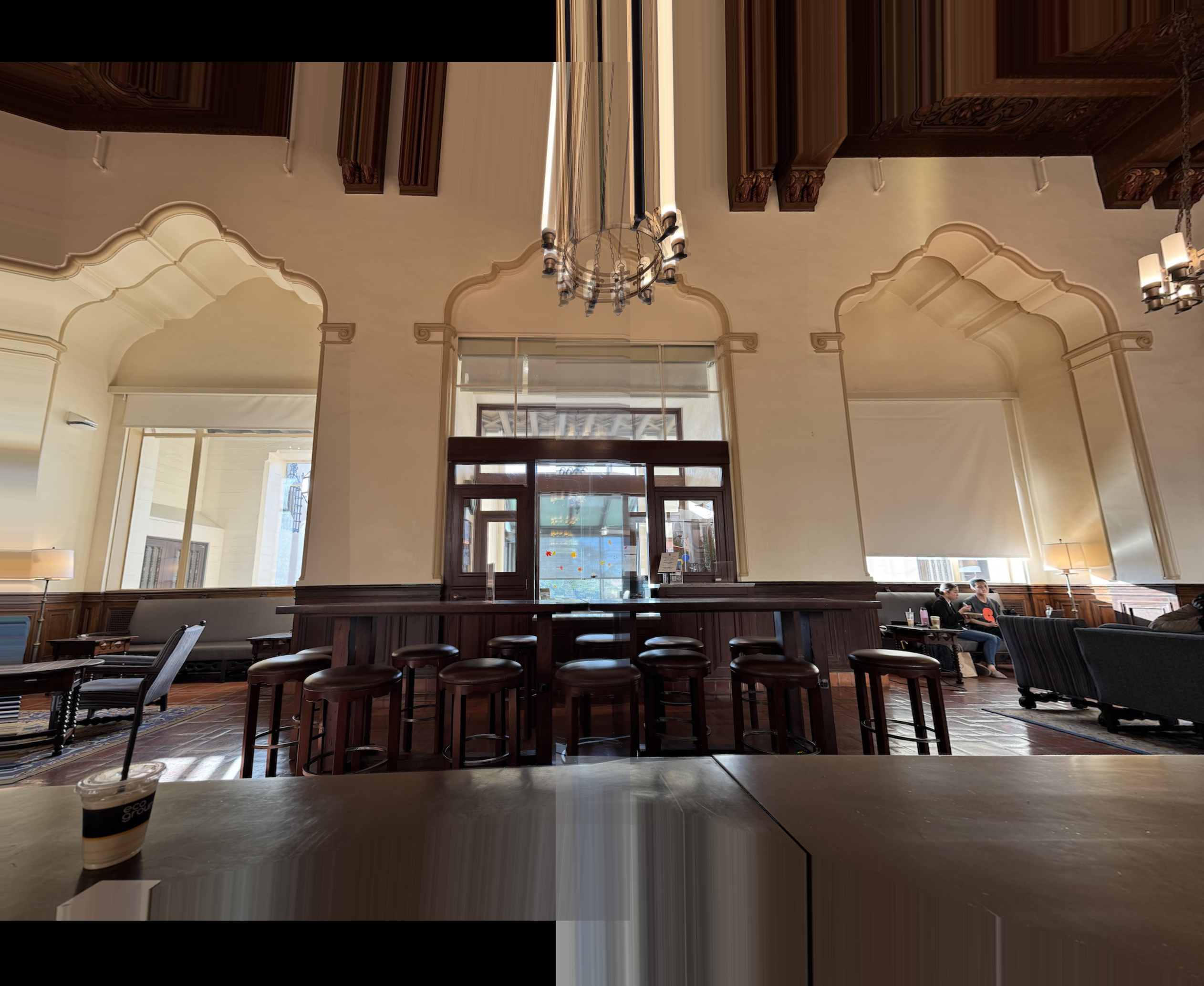
I repeated this process for 2 more sets of images: a courtyard and lounge hall within ihouse. As you can see, I did not end up travelling far to shoot.
Manual Results


Overall, this project was quite interesting, as well as challenging. I certainly learnt a lot about image warping and alignment, and how much harder it actually is to implement than I thought. The agony of manually selecting points, and then debugging the autostitching code for Part B of the project was definitely balanced out by the enjoyment of seeing somewhat decent panorama results. However, I do think that using a more robust method of blending would have produced even better panoramas.
Acknowledgements
This project is a course project for CS 180 at UC Berkeley. Part of the starter code is provided by course staff. This website template is referenced from Bill Zheng.